As I have elaborated some thoughts and the mathematic model I used in my last blog A Mathematic Model of Resource Sharing Problem. Now we can use this model to try to solve this problem. I have talked about the complexity of this problem, which make it very hard to get the global best solution. So I’m thinking about using a method, which is at least better than greedy algorithm, to see if it can make a difference on finding the best solution as possible. Mention: The best solution we found is not necessarily the global best.
Naturally, there’re some famous and popular methods come into my mind, such as annealing, genetic algorithm and Monte Carlo tree searching. Those algorithms have some features in common: they allow the program to sometimes preserve the situation which are not the best at that time. That’s why they always perform better compared with the greedy algorithm. To me, I’m more familiar with MCTS, so I decided to try this algorithm first.
Baseline
Apparently, we need some other algorithms as references. I chose 3 algorithms: Random sharing, greedy, enumerate. Random sharing randomly share for every tmp register, greedy choose the most common input of all branches to share, and enumerate try all sharing strategies to find the best one. So enumerate can always find the best sharing strategy, but its complexity is to high, so we can only use this algorithm as baseline in small scale problem.
Cost Function
After confirming 3 algorithms as baseline, we need to come up with a cost function to evaluate if a strategy is good or bad. Now I only take the amount of all mux’s input into consideration. So for example like:

Every row represents a branch, and every column represents an input. And the output can be written as o = tmp1 + tmp2. If we try the following sharing strategy.
branch1:
	tmp1 = a
branch2 & branch3:
	tmp1 = c
branch1 & branch2:
	tmp2 = b
branch3:
	tmp2 = d
The mux for tmp1 has two inputs a and c, and the mux for tmp2 has two inputs too. So the cost of this strategy is 2 + 2 = 4.
Monte Carlo Tree Searching
Monte Carlo Tree Searching, can also be called UCT if we use UCB to evaluate every situation. This algorithm is famous for being used in AlphaGo and beat the greatest human players. It based on
the famous Law of Large Numbers, which indicates that in the repeated occurrence of a large number of random events, it often presents an almost inevitable law. So computers can randomly simulate the Go game for many times and find the relatively accurate possibility of winning after taking a step. That’s why AlphaGo can beat all the human players, because it can see the development of the game in a long-term view, which let it barely make mistakes.
So, we can also use this principle to do resource sharing. We can also simulate to roughly calculate a sharing strategy’s cost. And we can choose the better one to keep on sharing. If you’re looking for the basic knowledge of MCTS, I suggest to take a look at this wikipedia page
Algorithm

Similar to the normal MCTS, we also have 4 steps. But each part make some modifications.
Selection:
While NOT ARRIVE LEAF:
	if node has child:
		if random(0,1) > 0.5 and node can explore:
			break
		else:
			node = the child with Higher Evaluation value
return node
In the selection step, we introduce UCB as an evaluation function. Every time, we choose the larger
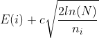
E(i) represents the value of a node, here is the countdown of the node’s cost, c is a constant number, N represents the visit time of the node’s parent , and n_i represents the visit time of the node itself. We can divide the parts before and after plus operator into two parts. The former one is called “exploitation”, it’s actually a greedy progress. Later one is called “exploration”, it helps MCTS to sometimes to explore the nodes which aren’t the best at present, but may become the best one in the future.
Expansion
After we choose a node from the selection step, we will expand this node. Generally speaking, is doing a “sharing step”, which is actually choose two column vectors of the matrix to do “or” and “and” operations. And the new situation become a child node of the chosen node.
Simulation
When we’ve generated a new child node, we need to simulate it to roughly evaluate it. The simulation process is simple, just randomly do “sharing steps” until the matrix cannot be shared (or use greedy method). And we can calculate the cost during this process.
Backpropagation
As we can see, the development of this Monte Carlo Tree is a non-symmetrical process. It will develop towards the direction which is more possible to get the better solutions. So when we expand and simulate a new node, we need to backpropagate its cost to its ancestors to help to select the direction to develop in the next loop.
The principle to backpropagate is a little different with the traditional MCTS. In this process, we’ll transfer the child’s simulation cost to its ancestor, and if the simulation cost is less than the ancestors’ cost, then overlap the ancestors’ cost. This means the child’s may have a better sharing strategy with less cost, and if we go through from the root node to this child node, we may probably find a better strategy. So we need to let this possibility visible during our early selection process by overlapping the ancestors’ cost.
Make decision
After we’ve developed a MCT in a limited time, we need to find the best sharing strategy from this tree. There’re two steps I took. First, we use a variable to store the best sharing strategy with least cost. If we arrive the leaf node whose matrix can’t be shared anymore, we’ll compare its cost with the stored one, and decide if the stored one is needed to be updated. Secondly, if we find the searching process haven’t arrived any leaf node which can’t be shared anymore, we’ll do a selection process from the root node. But the differences are that we will not expand any node, and the principle to choose only base on the cost (or cost + visit / parent.visit). Once we choose the node, we’ll use a simple enumerate / greedy method to share.
Overall Algorithm
After introducing four steps above, we can generate an overall algorithm.
While NOT SATISFY STOP CONDITION:
	node = Selection()
	if node is expandable:
		child = Expand(node)
		Simulate(child)
		Backpropagation(child)
MakeDecision()
Example
Assume we have such a matrix:

we can generate a MCT, and the matrix above represents the root node. Start the loop.
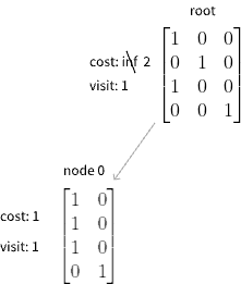
First we select the root node, and the root doesn’t have any child, so we expand it. We get the matrix:

And then we use greedy method to simulate it, we get its cost is 1. Then we backpropagate to the root, and update its cost. Mention: root need 1 sharing step to get to node 0, so its cost need to add 1
The next time we enter the loop we find the root has a child. Assume the random number in selection step is less than 0.5, so we choose node0 to expand, and get a child with a empty matrix. So its simulated cost is apparently zero, and when this cost spread to node 0, the cost add 1 is not less than the cost node 0 have, so no need to continue updating upwards. And because we’ve arrived at a state which can’t be shared anymore(empty matrix), we can record this state

Then we restart the loop again. We get a random number larger than 0.5, so we expand the root:

Restart the loop. This time, we find though node0 and node2 have the same cost, but node2 was only visited for once, so due to the UCB formula, we choose node2 to expand this time. Then we get:

Assume the program stop at this time, then the best sharing strategy is the state we stored before. It’s the node 1. So the sharing steps are: root - node0 - node1.
The original matrix (root matrix) is equal to this code:
if (state == 0) begin
	o = a;
end
else (state == 1) begin
	o = b;
end
else (state == 2) begin
	o = a;
end
else begin
	o = c;
end
and shared result is:
if (state == 0 && state == 2) begin
	tmp = a;
end
else (state == 1) begin
	tmp = b;
end
else begin
	tmp = c;
end
o = tmp
So this circuit at least needs a 3 input mux to implement.
Hyper Parameters
The constant c in selection, the condition in selection: if random(0,1) > 0.5 and node can explore:, the simulation method (random / greedy) and the evaluation method in make decision: cost / cost + parent.visit/ visit.
Presently I tried different combination of those hyper parameters, but the differences between those are not so apparent.
Batch test
I use python3 to finish the baseline algorithms and MCTS, and generate random cases to test. I first randomly generate the matrices’ scale (m, n and c),m ranges from 2 to 7, n ranges from 3 to 12 and c ranges from 2 to n. This means the codes which matrices represent have m branches, n inputs and c operators. Then generate 200 cases for each single scale. Then I calculate the total cost for those cases by running different algorithms.
The horizontal axis means m*n*(n-c), this can indicates the matrices’ scale. And the vertical axis means the total cost of 200 cases by using greedy minus total cost by using the other algorithms. Here the time limitation of MCTS is 0.5 s.

Greedy minus Random

Greedy minus MCTS

Greedy minus MCTS with random in selection

Greedy minus MCTS with count visit in make decision

Greedy minus MCTS with both count visit in make decision and random in selection
Apparently, MCTS is better than the popular greedy algorithm. What’s more, this algorithm is stable if we provide it sufficient time. For a medium size case, 0.5 s is totally enough. If we rewrite the code into cpp, the running time can be even shorter.
And I also did some comparison between enumerate and MCTS in smaller cases, which are m ranges from 2 to 7, n ranges from 3 to 7 and c ranges from 2 to n. The reason why I don’t compare enumerate with other algorithms in larger scale problems is because its complexity makes the program can’t finish even after few hours.

Enumerate minus Random

Enumerate minus Greedy

Enumerate minus MCTS

Enumerate minus MCTS with random in selection

Enumerate minus MCTS with count visit in make decision

Enumerate minus MCTS with both count visit in make decision and random in selection
Apparently, we can see in smaller cases, MCTS barely can make as good decisions as the Enumerate method, and better than other methods.
Conclusion
In a nutshell, the result of MCTS method is without doubt exciting and interesting. But we still need some real circuits and run some test in some design tools, like Design Compiler, to actually see its results under real circumstances. I have faith in it! Those test works will be done in the near future.
Cherry Young
A Undergraduate student from TsingHua University. Now doing some researches about Resource Sharing Algorithm in EDA, meanwhile working as an intern in an EDA company. Looking forward to become a master or PhD in 2023. Please contact me if you're willing to provide me an opportunity ^_^.
